Central Limit Theorem Simulation

16 Nov 2020 ~3 min read

Synopsis

This project will investigate the exponential distribution in R and compare it with the Central Limit Theorem. The exponential distribution can be simulated in R with rexp(n, lambda) where lambda is the rate parameter. The mean of exponential distribution is 1/lambda and the standard deviation is also 1/lambda. Set lambda = 0.2 for all of the simulations. Then, investigate the distribution of averages of 40 exponentials.

Illustrate via simulation and associated explanatory text the properties of the distribution of the mean of 40 exponentials. This is the criteria of the project :

Show the sample mean and compare it to the theoretical mean of the distribution.
Show how variable the sample is (via variance) and compare it to the theoretical variance of the distribution.
Show that the distribution is approximately normal.

In point 3, focus on the difference between the distribution of a large collection of random exponentials and the distribution of a large collection of averages of 40 exponentials of a thousand simulations.

Prepare the Simulation

set variables as defined in parameters of the exponential simulation.

# set variables according to parameters
simulation <- 1000
n <- 40
lambda <- 0.2

# set seed
set.seed(11)

# Create matrix of 1000 observation and 40 variable
data <- matrix(data = rexp(n * simulation, lambda), nrow = simulation)

Calculate the mean of simulation data for each column

rowMeanSim <- rowMeans(data)

Sample vs. Theoretical

Mean

Calculating the sample data mean, the average of 1000 simulations over 40 variables and the theoretical mean, the expected mean = 1/lambda.

# Calculate Simulation Mean
meanSimulation <- mean(rowMeanSim)
round(meanSimulation,3)

4.987

# Calculate Theoretical Mean
meanTheore <- 1/lambda
meanTheore

From this results, we know that the sample mean is 4.987 and the theoretical mean is 5. The comparation of the sample mean and theoretical mean is close.

Variance

Calculating how variable the distribution of sample is and compare it to the theoretical variance as expected.

# Calculating sample variance
varSimulation <- var(rowMeanSim)
round(varSimulation,3)

0.651

# Calculatiing theoretical variance
varTheore <- (1/lambda)^2/n
varTheore

0.625

As we can see, the sample variance and the theoretical variance is also close, with 0.651 for the sample and 0.625 for the theoretical.

Distribution

Comparing the simulation values and the theoretical values.

library(ggplot2)

plotSimulation <- data.frame(rowMeanSim)

ggplot(plotSimulation, aes(x = rowMeanSim)) + 
     geom_histogram(aes(y = ..density..), color = "black", fill = "lightgreen") +
     labs(title = "The Distribution of Average of Simulation in Exponential Data", 
          x = "Exponential Averages", y = "Density") +
     geom_vline(aes(xintercept = meanSimulation, colour = "black"), size = .8, show.legend = F) +
     geom_vline(aes(xintercept = meanTheore, colour = "red"), size = .8, show.legend = F) +
     stat_function(fun = dnorm, size = 1, color = "purple", args = list(meanSimulation, varSimulation)) +
     stat_function(fun = dnorm, size = 1, color = "orange", args = list(meanTheore, varTheore))

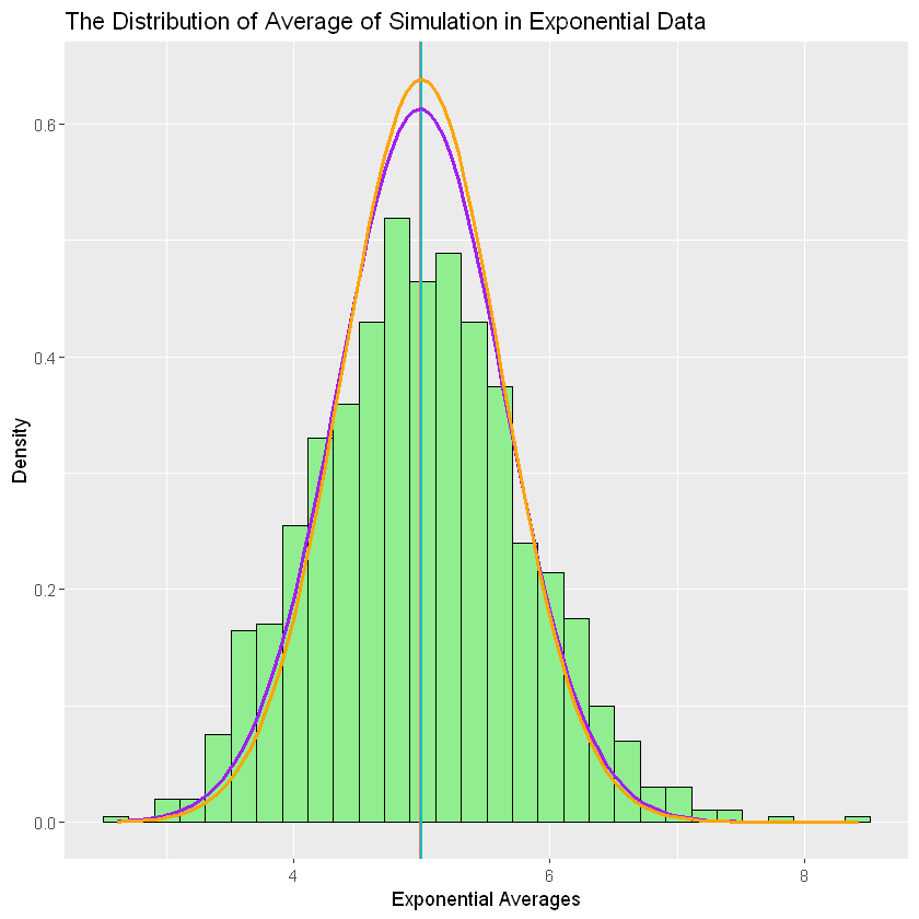
The density of the simulation data is shown by the “light green” bar. The vertical line is referred to the mean of the data. The color supposed to be “black” for simulation data and “red” for theoretical data, but both are so close and overlap. Then, The curve line is referred to the mean and variance of both. The simulation data shown by “purple” line. While, the theoretical data shown by “orange’ line.

As we see on the figure above, the distribution of the simulation means (“purple” line curve) is approximately close as the theoretical means distribution (“orange” line curve). These mean that the simulation data is consistent to Central Limit Theorem.