Electric Power Consumption

28 Sep 2020 ~4 min read

Synopsis

Introduction

This assignment uses data from the UC Irvine Machine Learning Repository, a popular repository for machine learning datasets. In particular, we will be using the “Individual household electric power consumption Data Set” which I have made available on the course web site:

Dataset: Electric power consumption [20MB]
Description: Measurements of electric power consumption in one household with a one-minute sampling rate over a period of almost 4 years. Different electrical quantities and some sub-metering values are available. The detailed description of these dataset could be obtained in UCI website.

Our overall goal here is simply to examine how household energy usage varies over a 2-day period in February, 2007. The task is to reconstruct the plots provided by lecturer, all of which were constructed using the base plotting system.

Processing Steps

Loading the data. Note that the dataset missing vaules are coded as ?.
Subsetting the dates to 2007-02-01 and 2007-02-02.
Converting date & time variables to Date/Time classes in R using strptime() and/or as.Date() functions.
Construct the plot and save it to a PNG file with 480x480 px size.

Loading the Data

# Download the Data set
    fileurl <- 'https://d396qusza40orc.cloudfront.net/exdata%2Fdata%2Fhousehold_power_consumption.zip'
    download.file(fileurl, destfile = 'household_power_consumption.zip')
      
# Unzip the Data set
    unzip('./household_power_consumption.zip')

# Read data from local directory
     rawData <- read.table('./household_power_consumption.txt', header = T,sep = ';', na.strings = '?')

print(paste("Observation: ", nrow(rawData),"Column: ", ncol(rawData)))
head(rawData)

[1] "Observation:  2075259 Column:  9"

Date	Time	Global_active_power	Global_reactive_power	Voltage	Global_intensity	Sub_metering_2	Sub_metering_3
16/12/2006	17:24:00	4.216	0.418	234.84	18.4	1	17
16/12/2006	17:25:00	5.360	0.436	233.63	23.0	1	16
16/12/2006	17:26:00	5.374	0.498	233.29	23.0	2	17
16/12/2006	17:27:00	5.388	0.502	233.74	23.0	1	17
16/12/2006	17:28:00	3.666	0.528	235.68	15.8	1	17
16/12/2006	17:29:00	3.520	0.522	235.02	15.0	2	17

# Subset data from 2007-02-01 and 2007-02-02
     data <- subset(rawData, Date == '1/2/2007' | Date == '2/2/2007')

# Correct date and time variable to the correct class
     data$Date <- as.Date(data$Date, format = '%d/%m/%Y')

# Add new variable called DateTime, consist of Variable Date and Time
     dateTime <- paste(data$Date, data$Time)
     data$DateTime <- strptime(dateTime, tz = "", '%Y-%m-%d %H:%M:%S')

str(data)
head(data)

'data.frame':	2880 obs. of  10 variables:
 $ Date                 : Date, format: "2007-02-01" "2007-02-01" ...
 $ Time                 : Factor w/ 1440 levels "00:00:00","00:01:00",..: 1 2 3 4 5 6 7 8 9 10 ...
 $ Global_active_power  : num  0.326 0.326 0.324 0.324 0.322 0.32 0.32 0.32 0.32 0.236 ...
 $ Global_reactive_power: num  0.128 0.13 0.132 0.134 0.13 0.126 0.126 0.126 0.128 0 ...
 $ Voltage              : num  243 243 244 244 243 ...
 $ Global_intensity     : num  1.4 1.4 1.4 1.4 1.4 1.4 1.4 1.4 1.4 1 ...
 $ Sub_metering_1       : num  0 0 0 0 0 0 0 0 0 0 ...
 $ Sub_metering_2       : num  0 0 0 0 0 0 0 0 0 0 ...
 $ Sub_metering_3       : num  0 0 0 0 0 0 0 0 0 0 ...
 $ DateTime             : POSIXlt, format: "2007-02-01 00:00:00" "2007-02-01 00:01:00" ...

	Date	Time	Global_active_power	Global_reactive_power	Voltage	Global_intensity	DateTime
66637	2007-02-01	00:00:00	0.326	0.128	243.15	1.4	2007-02-01 00:00:00
66638	2007-02-01	00:01:00	0.326	0.130	243.32	1.4	2007-02-01 00:01:00
66639	2007-02-01	00:02:00	0.324	0.132	243.51	1.4	2007-02-01 00:02:00
66640	2007-02-01	00:03:00	0.324	0.134	243.90	1.4	2007-02-01 00:03:00
66641	2007-02-01	00:04:00	0.322	0.130	243.16	1.4	2007-02-01 00:04:00
66642	2007-02-01	00:05:00	0.320	0.126	242.29	1.4	2007-02-01 00:05:00

Making Plots

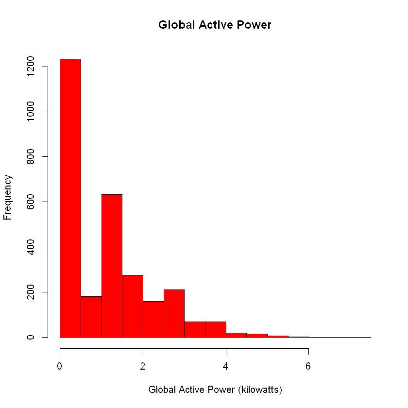
Plot 1

# Construct plot and save it to PNG file
     hist(data$Global_active_power,
          col = 'red',
          xlab = 'Global Active Power (kilowatts)',
          main = 'Global Active Power')
     
     dev.copy(png, 'plot1.png', height = 480, width = 480)
     dev.off()

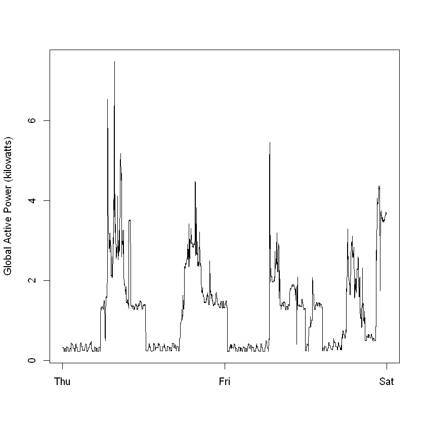
Plot 2

# Construct plot and save it to PNG file
     plot(data$DateTime,
          data$Global_active_power,
          type = 'l',
          ylab = 'Global Active Power (kilowatts)', 
          xlab = "")
     
     dev.copy(png, 'plot2.png', width = 480, height = 480)
     dev.off()

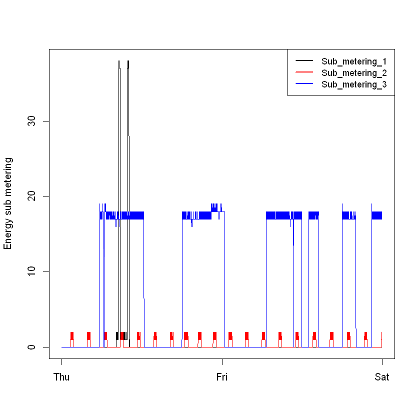
Plot 3

# Construct plot and save it to PNG file
     plot(data$DateTime, 
          data$Sub_metering_1,
          type = 'l', xlab = '',
          ylab = 'Energy sub metering')
     points(data$DateTime, 
            data$Sub_metering_2, 
            col = 'red', type = 'l')
     points(data$DateTime,
            data$Sub_metering_3,
            col = 'blue', type = 'l')
     legend('topright',c('Sub_metering_1', 'Sub_metering_2', 'Sub_metering_3'),
            col = c('black', 'red', ' blue'),
            lty = 1, lwd = 2, cex = 0.9)
     
     dev.copy(png, 'plot3.png', width = 480, height = 480)
     dev.off()

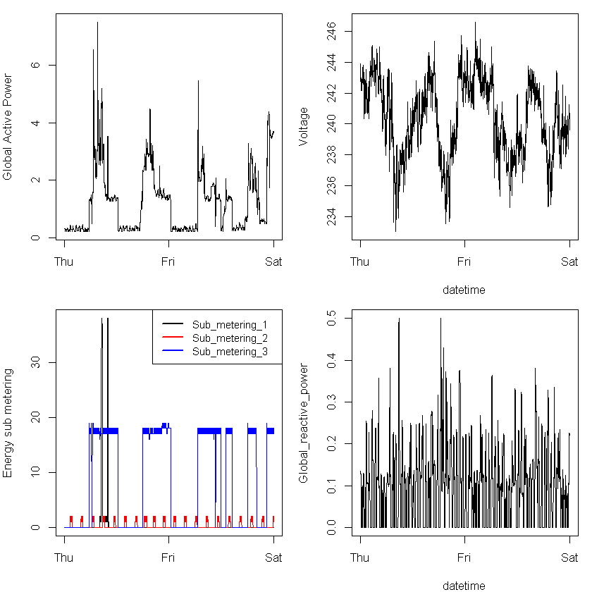
Plot 4

# Construct plot and save it to PNG file
     par(mfrow = c(2,2), mar = c(4,4,1,1))
     
     with(data, plot(DateTime, Global_active_power, type = 'l',
                        xlab = '', ylab = 'Global Active Power'))
     
     with(data, plot(DateTime, Voltage, type = 'l',
                        xlab = 'datetime',
                        ylab = 'Voltage'))
     
     with(data,{
          plot(DateTime, Sub_metering_1, type = 'l',
               xlab = '', ylab = 'Energy sub metering')
          lines(DateTime, Sub_metering_2, col = 'red')
          lines(DateTime, Sub_metering_3, col = 'blue')
          legend('topright', c('Sub_metering_1', 'Sub_metering_2', 'Sub_metering_3'),
                 col = c('black', 'red','blue'), lty = 1, lwd = 2, cex = 0.9)})
     
     with(data,
          plot(DateTime, Global_reactive_power,
               type = 'l', xlab = 'datetime',
               ylab = 'Global_reactive_power'))
     
     dev.copy(png, 'plot4.png', width = 480, height = 480)
     dev.off()