PM₂.₅ Emissions Data

Synopsis

Data

Fine particulate matter (PM\( _{2.5} \)) is an ambient air pollutant for which there is strong evidence that it is harmful to human health. In the United States, the Environmental Protection Agency (EPA) is tasked with setting national ambient air quality standards for fine PM and for tracking the emissions of this pollutant into the atmosphere. Approximatly every 3 years, the EPA releases its database on emissions of PM\( _{2.5} \). This database is known as the National Emissions Inventory (NEI). You can read more information about the NEI at the EPA National Emissions Inventory web site.

For each year and for each type of PM source, the NEI records how many tons of PM\( _{2.5} \) were emitted from that source over the course of the entire year. The data that you will use for this assignment are for 1999, 2002, 2005, and 2008.

The data for this assignment are available from the course web site as a single zip file:

• Data for Peer Assessment [29Mb]

The zip file contains two files:

PM\( _{2.5} \) Emissions Data (summarySCC_PM25.rds): This file contains a data frame with all of the PM\( _{2.5} \) emissions data for 1999, 2002, 2005, and 2008. For each year, the table contains number of tons of PM\( _{2.5} \) emitted from a specific type of source for the entire year.

Source Classification Code Table (Source_Classification_Code.rds): This table provides a mapping from the SCC digit strings in the Emissions table to the actual name of the PM\( _{2.5} \) source. The sources are categorized in a few different ways from more general to more specific and you may choose to explore whatever categories you think are most useful.

Assignments

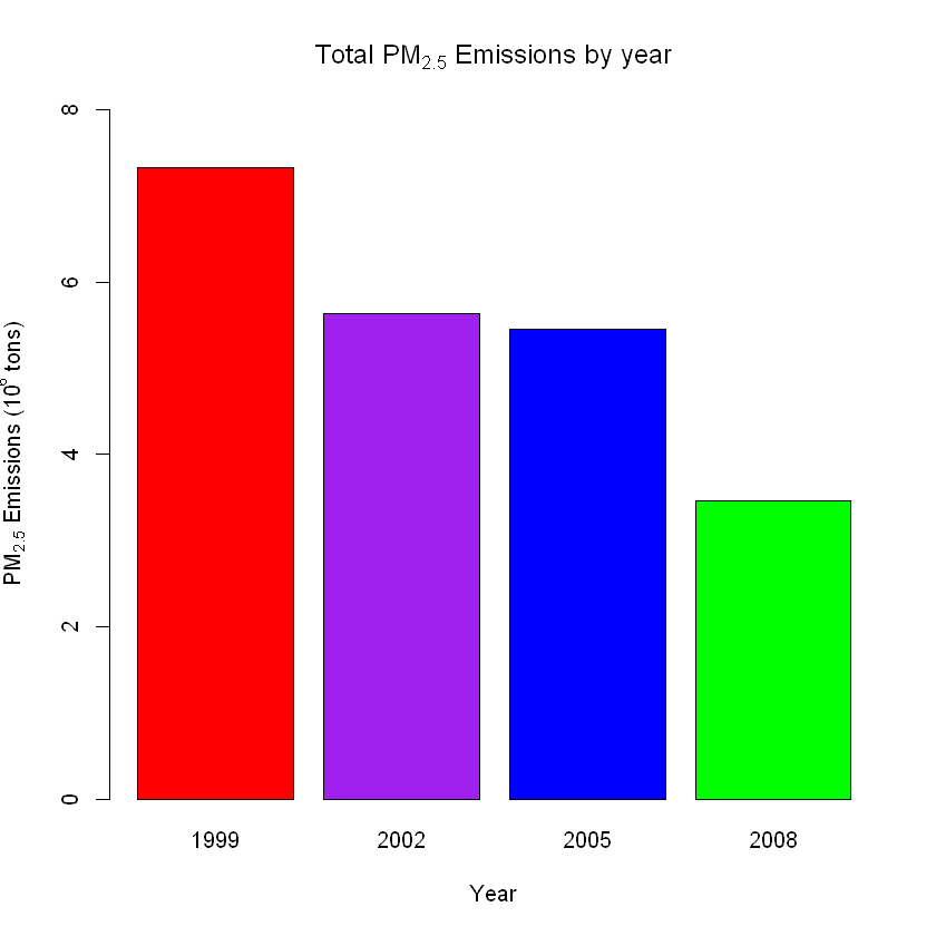
1. Have total emissions from PM\( _{2.5} \) decreased in the United States from 1999 to 2008? Using the base plotting system, make a plot showing the total PM\( _{2.5} \) emission from all sources for each of the years 1999, 2002, 2005, and 2008.

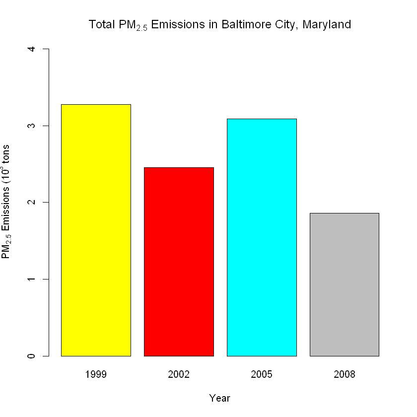
2. Have total emissions from PM\( _{2.5} \) decreased in the Baltimore City, Maryland (fips == "24510") from 1999 to 2008? Use the base plotting system to make a plot answering this question.

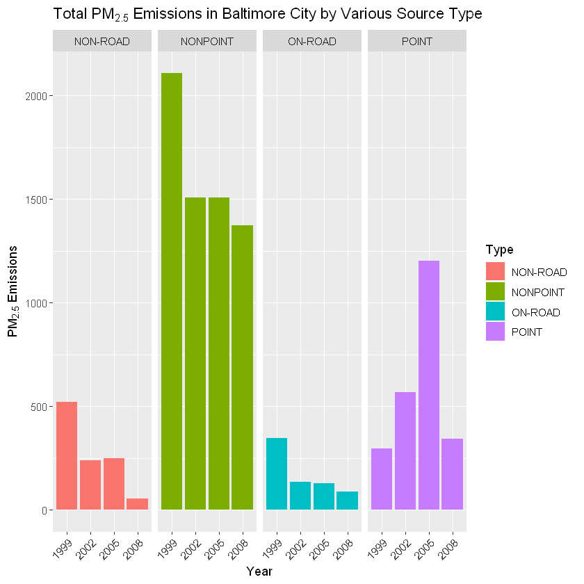
3. Of the four types of sources indicated by the type (point, nonpoint, onroad, nonroad) variable, which of these four sources have seen decreases in emissions from 1999–2008 for Baltimore City? Which have seen increases in emissions from 1999–2008? Use the ggplot2 plotting system to make a plot answer this question.

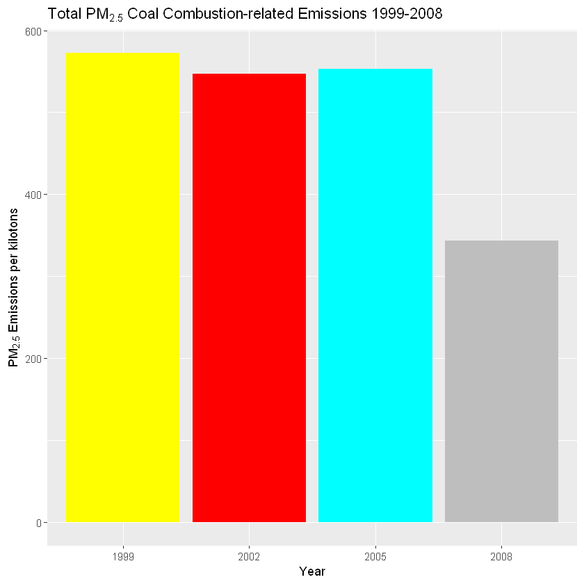
4. Across the United States, how have emissions from coal combustion-related sources changed from 1999–2008?

5. How have emissions from motor vehicle sources changed from 1999–2008 in Baltimore City?

6. Compare emissions from motor vehicle sources in Baltimore City with emissions from motor vehicle sources in Los Angeles County, California (fips == "06037"). Which city has seen greater changes over time in motor vehicle emissions?

Loading the Data

# Download the Data set
    fileurl <- 'https://d396qusza40orc.cloudfront.net/exdata%2Fdata%2FNEI_data.zip'
    download.file(url = fileurl, destfile = "NEI_data.zip")

# Unzip the Data set
    unzip('./NEI_data.zip')

# Read data from local directory
    NEI <- readRDS('./summarySCC_PM25.rds')
    SCC <- readRDS('./Source_Classification_Code.rds')

Making Plots

1. Have total emissions from PM\( _{2.5} \) decreased in the United States from 1999 to 2008?

# Make new table with total emmission per year
    emissionByYear <- aggregate(Emissions ~ year, NEI, sum)
    color1 <- c('red', 'purple', 'blue', 'green')

# Create a barplot by using new table
    color1 <- c('red', 'purple', 'blue', 'green')

    barplot(
         (emissionByYear$Emissions)/10^6,
         xlab = 'Year',
         names.arg = emissionByYear$year,
         ylab = expression('PM'[2.5]*' Emissions (10'^6*' tons)'),
         ylim = c(0,8),
         main = expression('Total PM'[2.5]*' Emissions by year'),
         col = color1
    )

#Save the barplot to PNG file
    dev.copy(png, './plot1.png')
    dev.off()

2. Have total emissions from PM\( _{2.5} \) decreased in the Baltimore City, Maryland (fips == "24510") from 1999 to 2008?

# Subsetting the data to ONLY shows Baltimore and making a new table with total emissions per year
    baltimore <- subset(NEI, fips == '24510')
    emissionByYear <- aggregate(Emissions ~ year, baltimore, sum)

# Create a barplot by using new table
    with(emissionByYear, 
         barplot(Emissions/10^3,
                 names.arg = year,
                 xlab = 'Year',
                 ylab = expression('PM'[2.5]*' Emissions (10'^3*' tons'),
                 ylim = c(0,4),
                 main = expression('Total PM'[2.5]*' Emissions in Baltimore City, Maryland'),
                 col = year))

#Save the barplot to PNG file
    dev.copy(png, './plot2.png')
    dev.off()

3. Of the four types of sources indicated by the type (point, nonpoint, onroad, nonroad) variable, which of these four sources have seen decreases in emissions from 1999–2008 for Baltimore City? Which have seen increases in emissions from 1999–2008?

# Load necessary library
    library(ggplot2)

# Create a plot by using baltimore table
    ggplot(baltimore, aes(x = factor(year), y = Emissions, fill = type)) + 
            geom_bar(stat = 'identity') +
            facet_grid(.~type) +
            ggtitle(expression('Total PM'[2.5]*' Emissions in Baltimore City by Various Source Type')) + 
            xlab('Year') + 
            ylab(expression('PM'[2.5]*' Emissions')) +
            labs(fill = 'Type') +
            theme(axis.text.x = element_text(angle = 45, hjust = 1))

#Save the plot to PNG file
    dev.copy(png, './plot3.png')
    dev.off()

4. Across the United States, how have emissions from coal combustion-related sources changed from 1999–2008?

# Subsetting the data to ONLY shows emissions from coal combustion-related and making a new table
    coal <- grepl('Fuel Comb.*Coal', SCC$EI.Sector)
    coalSCC <- SCC[coal,]

    emissionByCoal <- subset(NEI, NEI$SCC %in% coalSCC$SCC)

# Create a barplot by using new table
    ggplot(emissionByCoal, aes(x = factor(year), y = Emissions/1000)) + 
            geom_bar(stat = 'identity', fill = emissionByCoal$year) +
            ggtitle(expression('Total PM'[2.5]*' Coal Combustion-related Emissions 1999-2008')) + 
            xlab('Year') + 
            ylab(expression('PM'[2.5]*' Emissions per kilotons'))

#Save the barplot to PNG file
    dev.copy(png,'./plot4.png')
    dev.off()

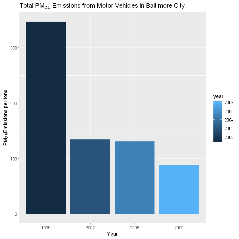
5. How have emissions from motor vehicle sources changed from 1999–2008 in Baltimore City?

# Subsetting the data to ONLY shows emissions from motor vehicle source in Baltimore and making a new table
    baltimoreVehicle <- subset(NEI, fips == '24510' & type == 'ON-ROAD')
    emissionByVehicle <- aggregate(Emissions ~ year, baltimoreVehicle, sum)

# Create a barplot by using new table
    ggplot(emissionByVehicle, aes(x = factor(year), y = Emissions, fill = year)) +
            geom_bar(stat = 'identity') +
            ggtitle(expression('Total PM'[2.5]*' Emissions from Motor Vehicles in Baltimore City')) +
            xlab('Year') +
            ylab(expression('PM'[2.5]*'Emissions per tons'))

#Save the barplot to PNG file
    dev.copy(png, './plot5.png')
    dev.off()

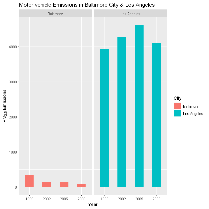
6. Compare emissions from motor vehicle sources in Baltimore City with emissions from motor vehicle sources in Los Angeles County, California (fips == "06037"). Which city has seen greater changes over time in motor vehicle emissions?

# Subsetting the data to ONLY shows emissions from motor vehicle source in Baltimore and Los Angeles
    baltimoreVehicle <- subset(NEI, fips == '24510' & type == 'ON-ROAD')
    laVehicle <- subset(NEI, fips == '06037' & type == 'ON-ROAD')

# Merge two table into one
    baltimoreVehicle$city <- 'Baltimore'
    laVehicle$city <- 'Los Angeles'
    emissionByVehicle <- rbind(baltimoreVehicle, laVehicle)


# Create a barplot by using new table
    ggplot(emissionByVehicle, aes(x = factor(year), y = Emissions, fill = city)) + 
                   geom_bar(stat = 'identity', width = 0.5) +
                   facet_grid(.~city) +
                   ggtitle('Motor vehicle Emissions in Baltimore City & Los Angeles') + 
                   xlab('Year') + 
                   ylab(expression('PM'[2.5]*' Emissions')) +
                   labs(fill = 'City')

#Save the barplot to PNG file
    dev.copy(png, './plot6.png')
    dev.off()

Summary

• Based on the barplot, total emission from PM\( _{2.5} \) in United Stated from 1999 to 2008 has been significantly decreased.
• Based on the barplot, total emission from PM\( _{2.5} \) in Baltimore City, Maryland from 1999 to 2008 has been fluctuative year by year.
• Of the four types of sources indicated by the type (point, nonpoint, onroad, nonroad) variable, nonpoint, onroad, and nonroad seems to decreasing, while on variable point were steadily increasing until 2005 and drop at 2008.
• Across the United States, emissions from coal combustion-related source are relatively stagnant until 2005, then significanly decreased at 2008.
• In Baltimore City, Maryland, emissions from motor vehicle sources are drop significantly from 1999 to 2002. However in 2002-2008, the total emissions from motor vehicle sources seems to be stagnant.
• Based on the barplot, Los Angeles County are way higher than Baltimore City in term of the total emissions from motor vehicle sources. Despite of that, Baltimore City has greater changes by decreasing total emissions over time.